A plain-language walk-through of the desktop application, from opening it for the first time to producing a result you can rerun and cite. No programming is needed for the normal workflow.
OffshoreLH2 is a desktop program. You describe an offshore hydrogen project in it: where the site is, what equipment you would install and how ships collect the hydrogen. The program then simulates a full year, hour by hour, and reports how much hydrogen reaches the customer, at what cost, and whether every physical check passed.
You will need
A Windows 10 or 11 computer (64-bit) or a Linux machine.
Python 3.12 or 3.13, CMake and a C++20 compiler; on Windows, Microsoft C++ Build Tools. The launcher script does the rest.
Access to the OffshoreLH2 repository, which is currently private. Ask for access.
Optional: a free Copernicus Climate Data Store account, for automatic ERA5 weather download.
Optional: an Ocean Networks Canada Oceans 3.0 token, for comparing ERA5 with ocean observations.
Tip. The repository includes a demonstration project, examples/canonical_baseline_2020.olh2, with one year of North Atlantic weather. It is the quickest way to see a complete run before setting up your own site.
02
Install and open the application
On Windows, open PowerShell in the repository folder and run:
Set-ExecutionPolicy -Scope Process -ExecutionPolicy Bypass -Force
.\scripts\run_gui_windows.ps1
The launcher finds a suitable Python, creates an isolated environment in .venv, builds the C++ core, installs the desktop interface and starts the application. The first build takes a few minutes; later launches are quick.
On Linux, run ./scripts/run_gui_linux.sh, or install with python -m pip install -e '.[gui]' and start the program with offshorelh2-gui.
For automatic ERA5 download and the Ocean Networks Canada comparison, also install the optional data packages:
.venv\Scripts\python -m pip install -e ".[data]"
03
Find your way around
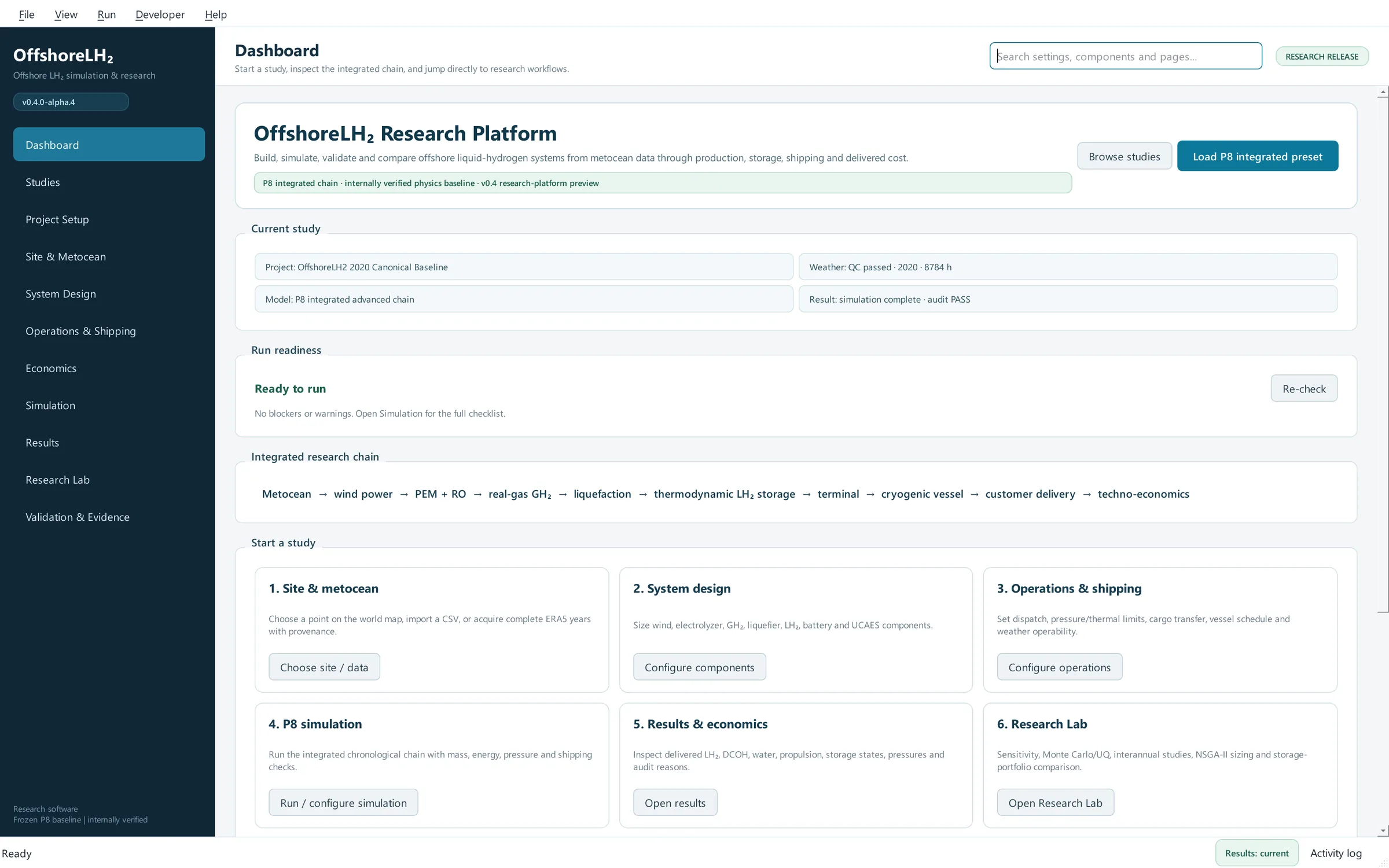
The sidebar on the left lists eleven pages in the order a study normally follows. The Dashboard shows the current project, weather status, active model and latest result, plus a Run readiness summary.
Start a study cards jump to each step.
Load P8 integrated preset switches on all of the higher-fidelity physics (real-gas hydrogen storage, LH₂ tank and vessel thermodynamics, thermodynamic compressed-air storage and electrolyzer ageing) without changing your equipment sizes or costs. It also switches the simulation to a single chronological year, because stack ageing cannot repeat.
The search box at the top (Ctrl+K) finds any setting, component or page and takes you straight to it.
The Dashboard: current study, readiness and shortcuts to every step.
04
Create and save a project
Choose File → New Project (Ctrl+N).
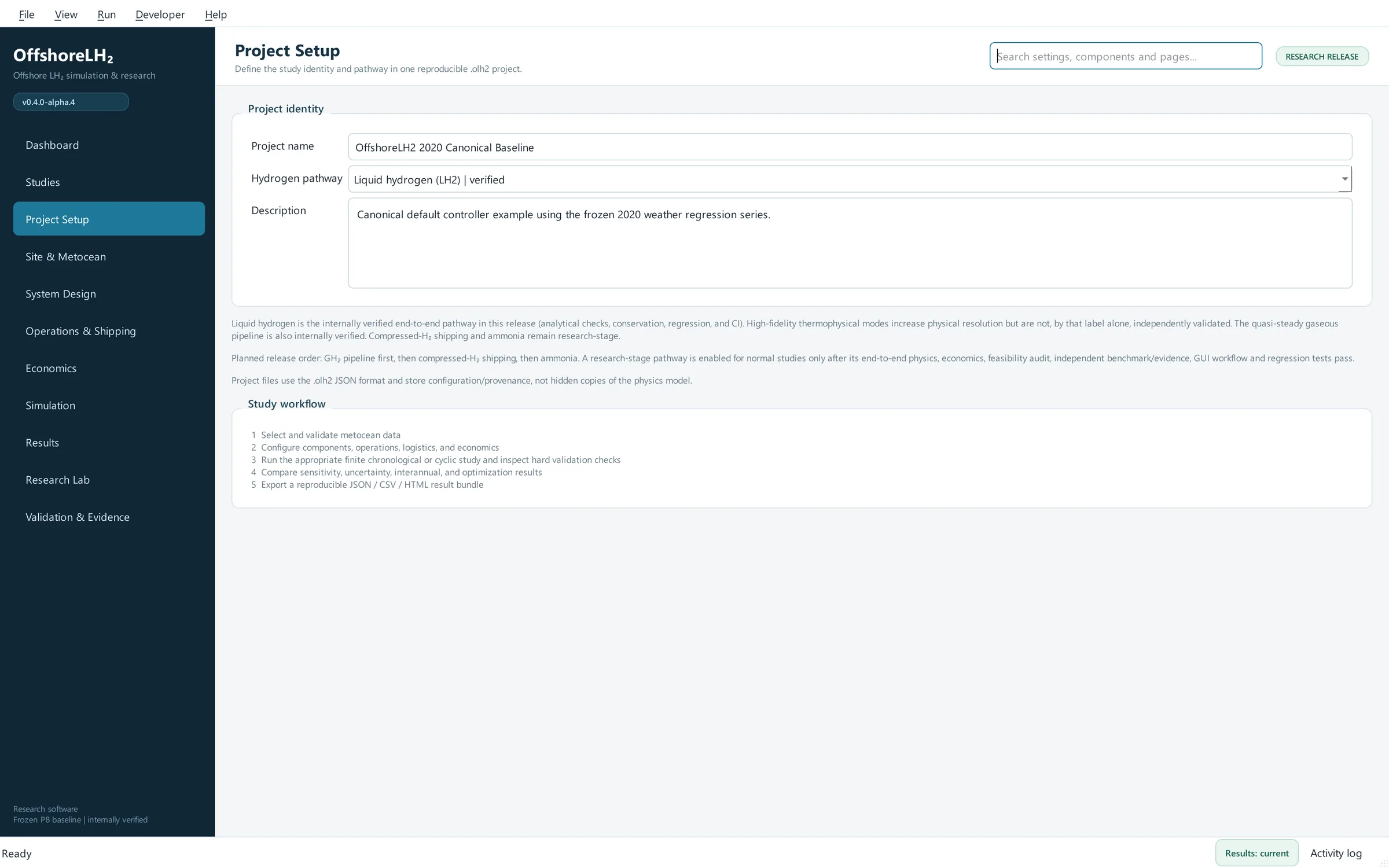
On Project Setup, give the study a descriptive name and a short description.
Choose the hydrogen pathway: liquid hydrogen shipped by vessel, or gaseous hydrogen through a pipeline. Research-stage pathways appear in the list but cannot be selected.
Save early with File → Save (Ctrl+S). Projects are stored as .olh2 files, readable JSON that records every setting.
An asterisk in the window title means there are unsaved changes. OffshoreLH2 asks before discarding them, and File → Open Recent lists your recent projects.
Project Setup: name, pathway and description. Research-stage pathways are visible but disabled.
05
Choose a site and prepare weather data
Every simulation needs hourly wind speed and significant wave height for at least one complete calendar year. There are two ways to provide them.
Option A: automatic preparation from ERA5
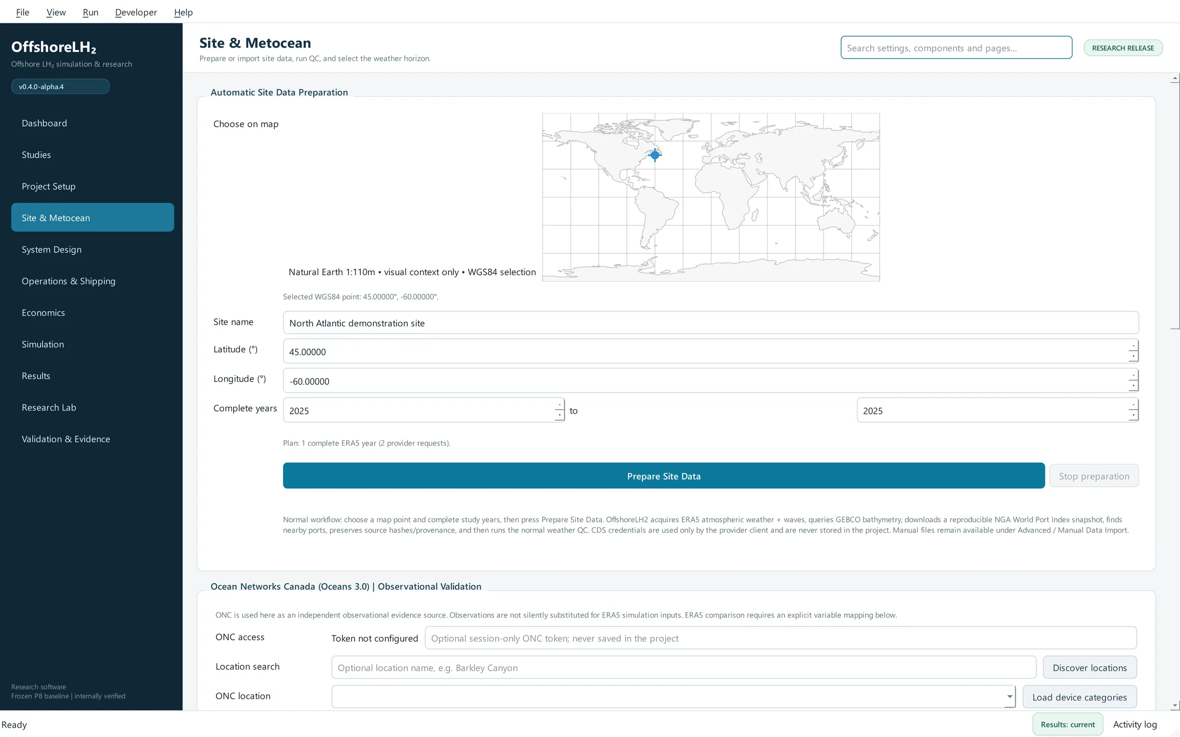
On Site & Metocean, click the world map or type the latitude and longitude. Scroll to zoom, drag to pan and double-click to reset.
Optionally name the site, then choose the first and last complete years.
Press Prepare Site Data. OffshoreLH2 downloads ERA5 wind and wave data, looks up water depth (GEBCO) and nearby ports (NGA World Port Index), records file hashes and provenance, and then runs quality control. Downloads are cached and can be stopped and resumed.
This needs a Copernicus Climate Data Store API key saved in a .cdsapirc file in your home folder. The key is used only by the download client and is never stored in the project.
Option B: your own CSV file
Open Advanced / Manual Data Import and choose an hourly CSV file with the columns timestamp, wind_speed_m_s and wave_height_m.
Quality control
Press Validate & select design year. The program rebuilds complete calendar years, rejects impossible values, fills only short gaps (6 hours by default), rejects years with longer gaps, corrects wind to hub height and selects a representative design year. The summary lists accepted and rejected years with reasons.
Optional. The Ocean Networks Canada panel finds ONC stations and instruments, previews observations and compares them with the loaded ERA5 series (bias, MAE, RMSE and correlation). Observations are used as evidence only and never replace the simulation weather. Supply the token through the ONC_TOKEN environment variable or the session-only field; it is never saved.
Site & Metocean: map-based site selection and automatic ERA5 preparation.
06
Design the system
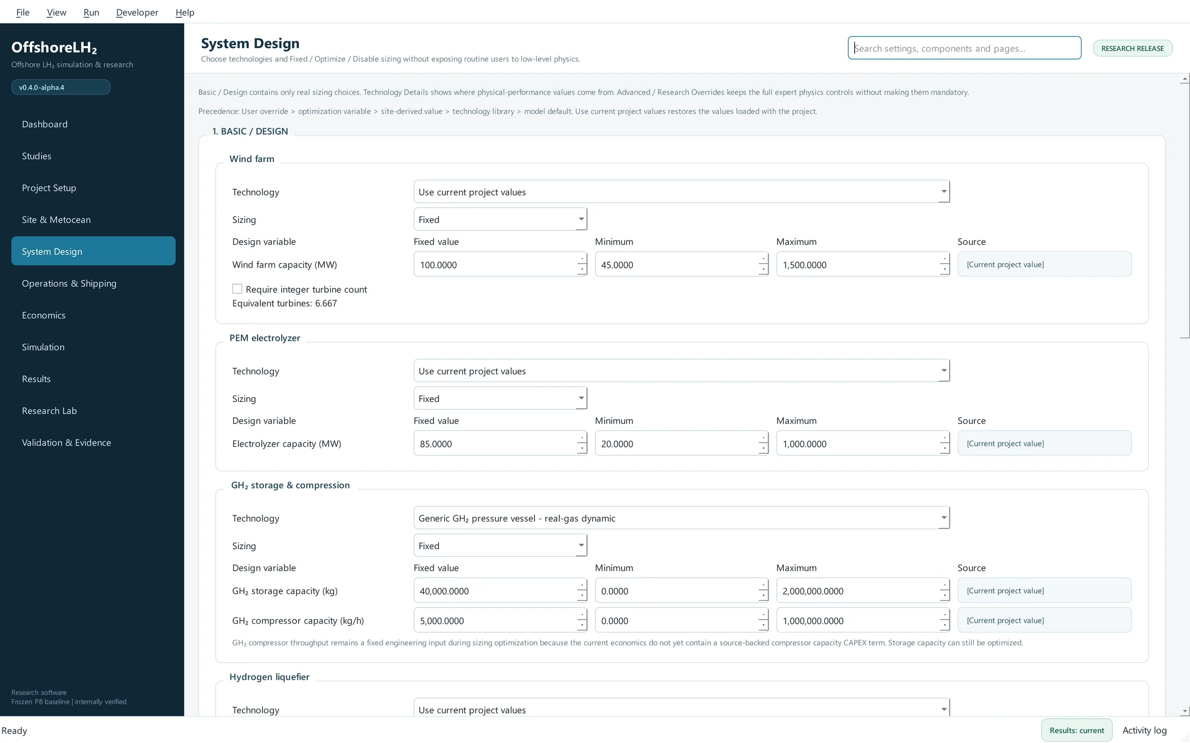
System Design lists each component: wind farm, PEM electrolyzer, hydrogen buffer and compressor, liquefier, LH₂ tank, battery and compressed-air storage. For each one:
Technology: keep Use current project values or pick a generic technology preset. Presets show where their numbers come from.
Sizing: Fixed uses one value, Optimize lets the optimizer search between a minimum and a maximum, and Disable removes the component.
Source: shows whether a value came from you, the optimizer, the site, a technology library or a model default.
Three levels keep the page manageable: Basic / Design for sizing, Technology Details for performance data and sources, and Advanced / Research Overrides for expert physics settings. Each detailed model carries a plain-language fidelity label explaining what the simpler version leaves out.
Tip. Start from the defaults and change one thing at a time. That makes it much easier to understand why a result changed.
System Design: technology, sizing mode, bounds and value source for every component.
07
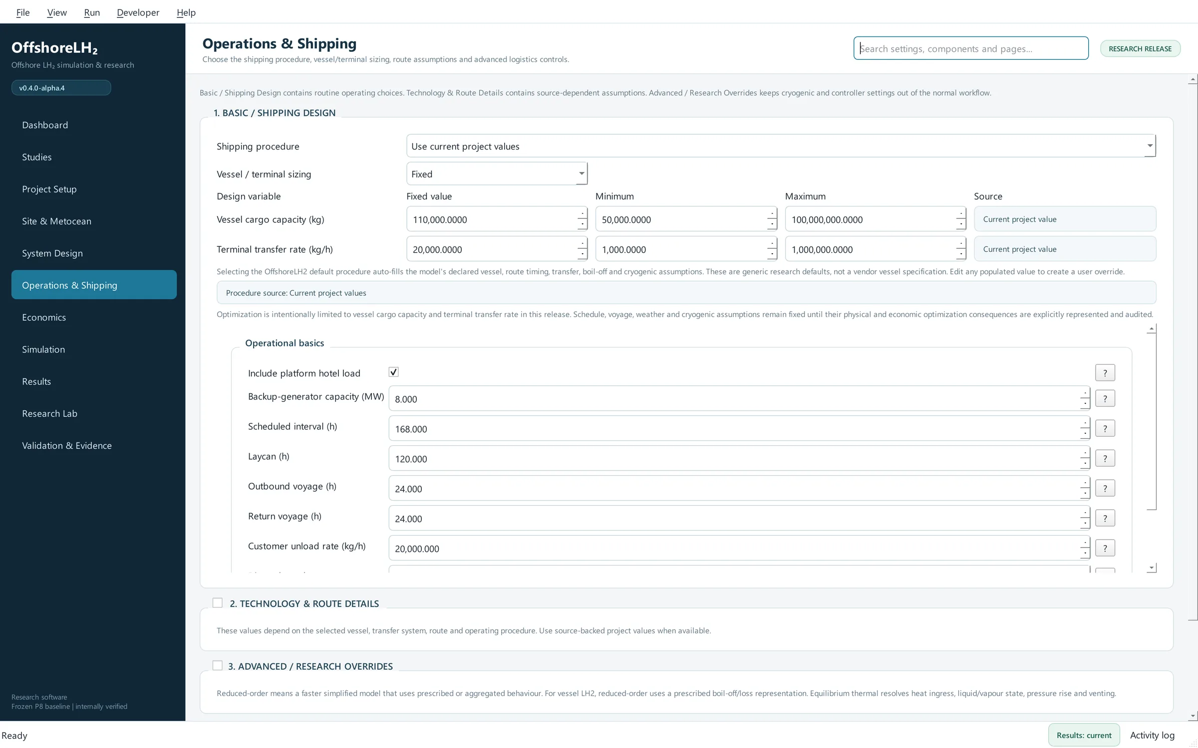
Set up operations and shipping
Operations & Shipping describes how the platform runs and how hydrogen leaves it:
Shipping procedure: the generic OffshoreLH2 procedure fills in declared research defaults for the vessel, voyage, transfer and boil-off. These are research defaults, not a vendor specification.
Vessel cargo capacity and terminal transfer rate can be Fixed or Optimize. Other logistics values stay fixed in this release.
Operational basics: platform hotel load, backup generator, call interval, laycan, voyage times and customer unloading rate.
Technology & Route Details and Advanced / Research Overrides hold transfer weather limits, cargo-tank thermodynamics, reliquefaction and controller settings.
The default dispatch order is battery first, then compressed-air storage. The Future optimized dispatch panel (MILP and MPC) is deliberately disabled, because those back-ends are not implemented yet.
Operations & Shipping: procedure, vessel and terminal sizing, and operating basics.
08
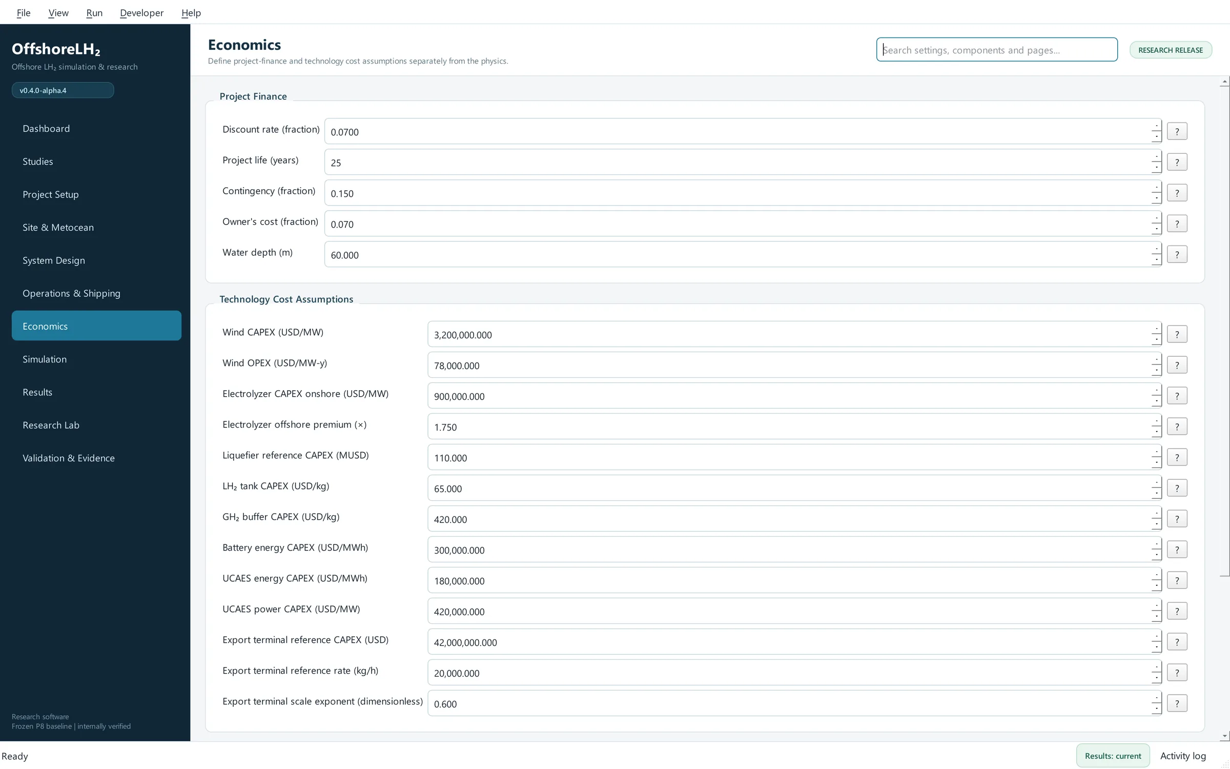
Enter cost assumptions
On Economics, set the financial parameters and the capital and operating costs of each technology. Economics is calculated outside the physics core, so financial assumptions never affect the physical simulation.
Results report the delivered cost of hydrogen (DCOH) at more than one boundary: at the offshore transfer point, including shipping, and at the customer. The default values are research assumptions that make the examples runnable. Replace them with project-specific data and record where each number came from.
Economics: financial and technology cost assumptions, kept separate from the physics.
09
Check readiness and run the simulation
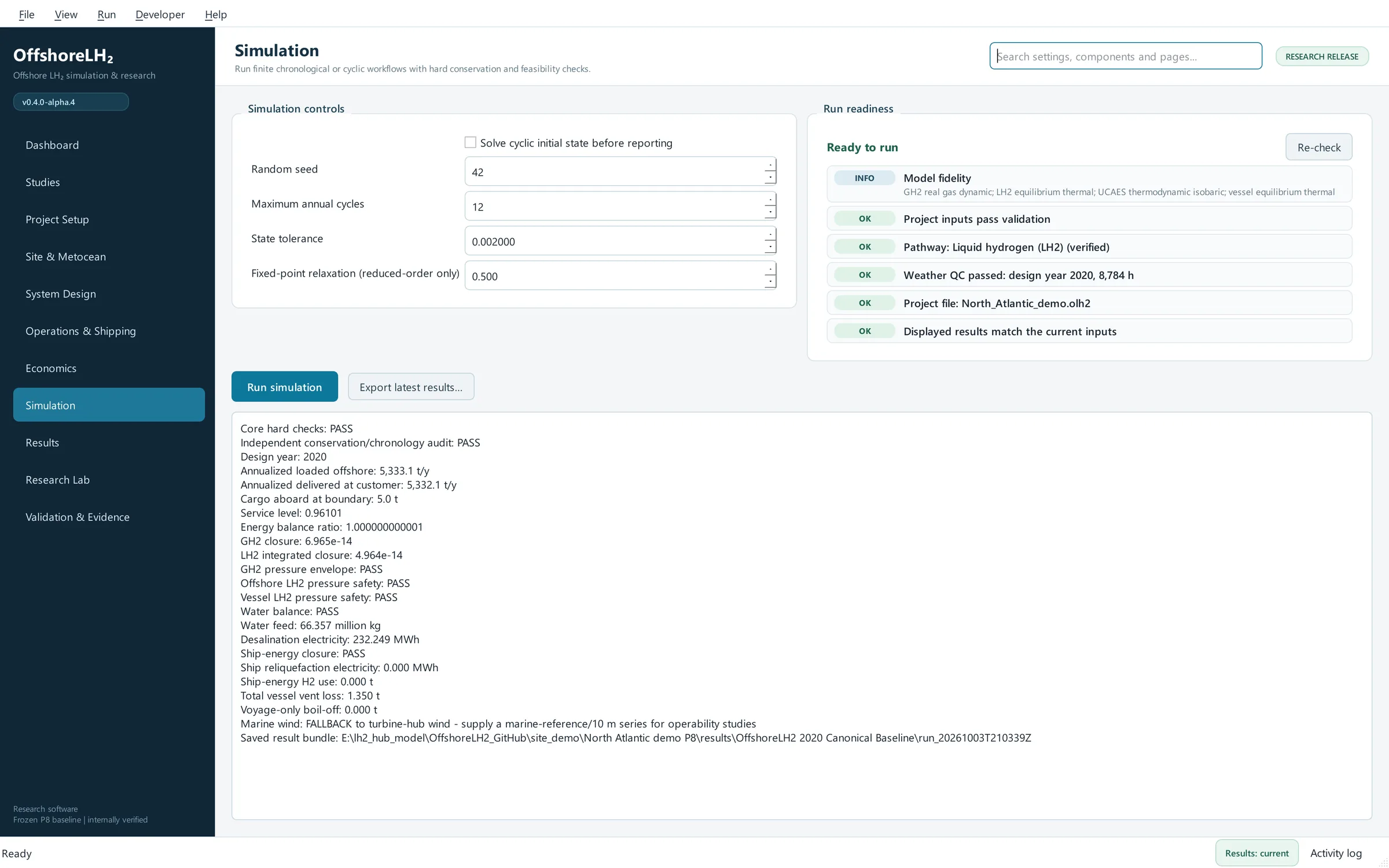
The Run readiness list on the Simulation page updates as you edit:
Blockers stop a run, for example a missing weather file or a combination of settings that cannot work together.
Review items do not stop a run but matter for interpretation, such as unsaved changes or stale results.
Each item has a Go to button that opens the setting to fix.
Then choose how the year is simulated:
Cyclic steady state (the "solve cyclic initial state" option) repeats the year until storage levels at the start and end agree, so results do not depend on an arbitrary starting inventory. Use it for periodic design studies.
Finite chronological runs the year once from a defined state. It is required when electrolyzer ageing is switched on, because stack age keeps increasing and cannot repeat.
Press Run simulation (F5). A reduced-order year takes a few seconds; the full higher-fidelity chain takes about a minute per year. Cancel run (Shift+F5) stops at the next safe checkpoint, and nothing partial is saved as a result.
A sound run report shows hard checks PASS, an independent audit PASS, an energy balance ratio of about 1 and very small hydrogen closure errors.
Simulation: readiness checks and the run report from a higher-fidelity run.
10
Read the results
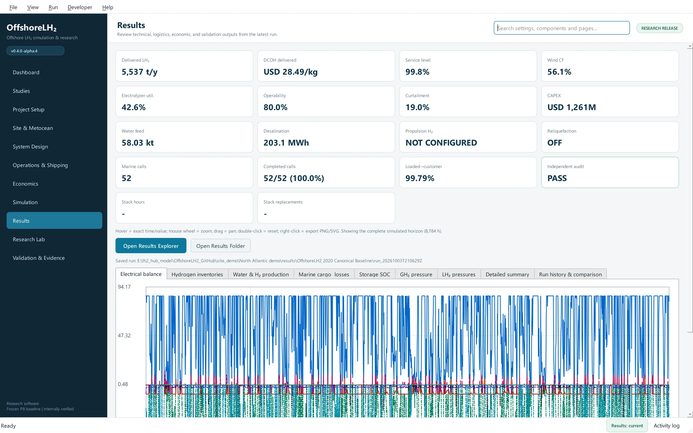
The Results page opens with key results: hydrogen delivered per year, delivered cost, service level (the share of requested hydrogen that was delivered), wind capacity factor, equipment utilization, marine operability, capital cost, water use, marine calls and the audit outcome.
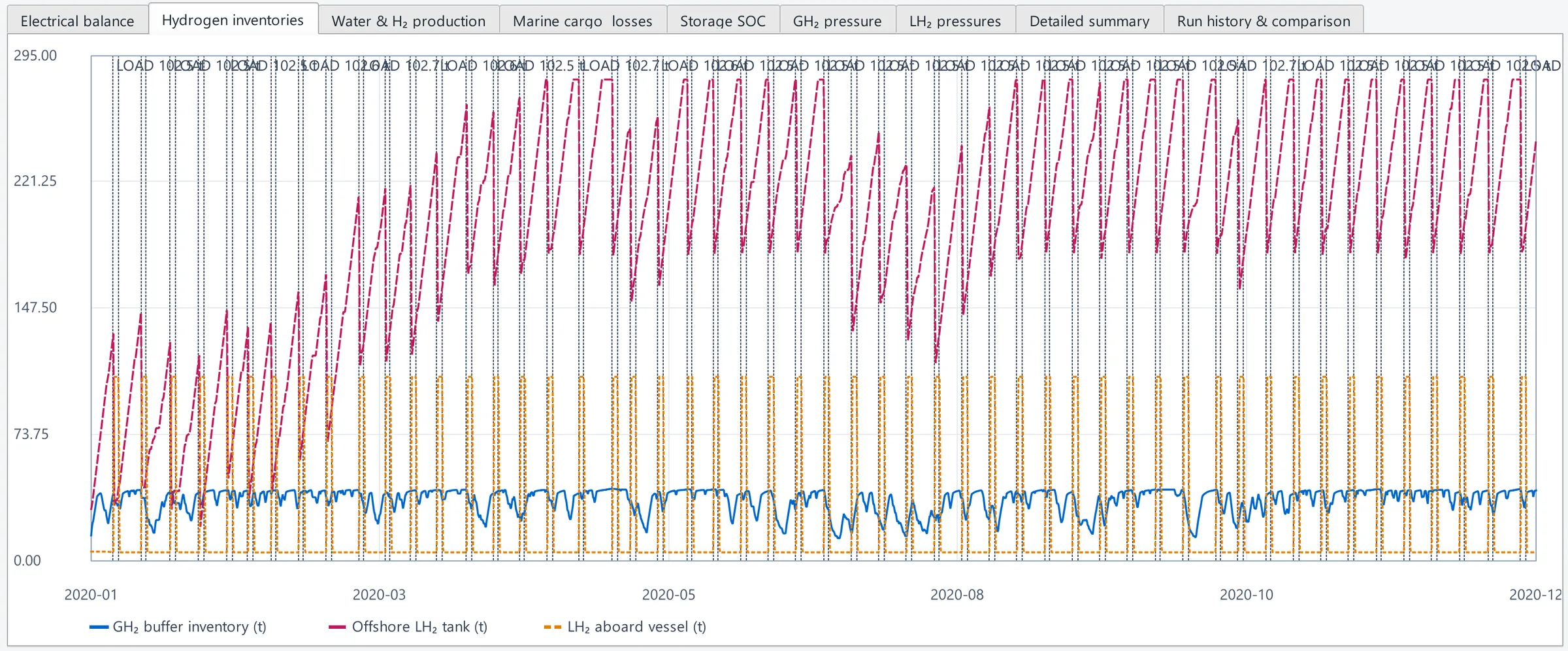
The chart tabs below show the full year hour by hour: electrical balance, hydrogen inventories, water and hydrogen production, marine cargo and losses, storage state of charge, and gas and liquid hydrogen pressures. Hover for exact values; scroll to zoom, drag to pan, double-click to reset and right-click to export a chart as PNG or SVG. Open Results Explorer opens the same saved run in a local browser view with more detail.
If you change any input after a run, a stale results banner names what changed. Run again before exporting or citing numbers.
Results: key figures for the demonstration case, with chart tabs below.Hydrogen inventories through the year: the offshore LH₂ tank fills between vessel calls and empties at each loading.
11
Compare runs and cite them
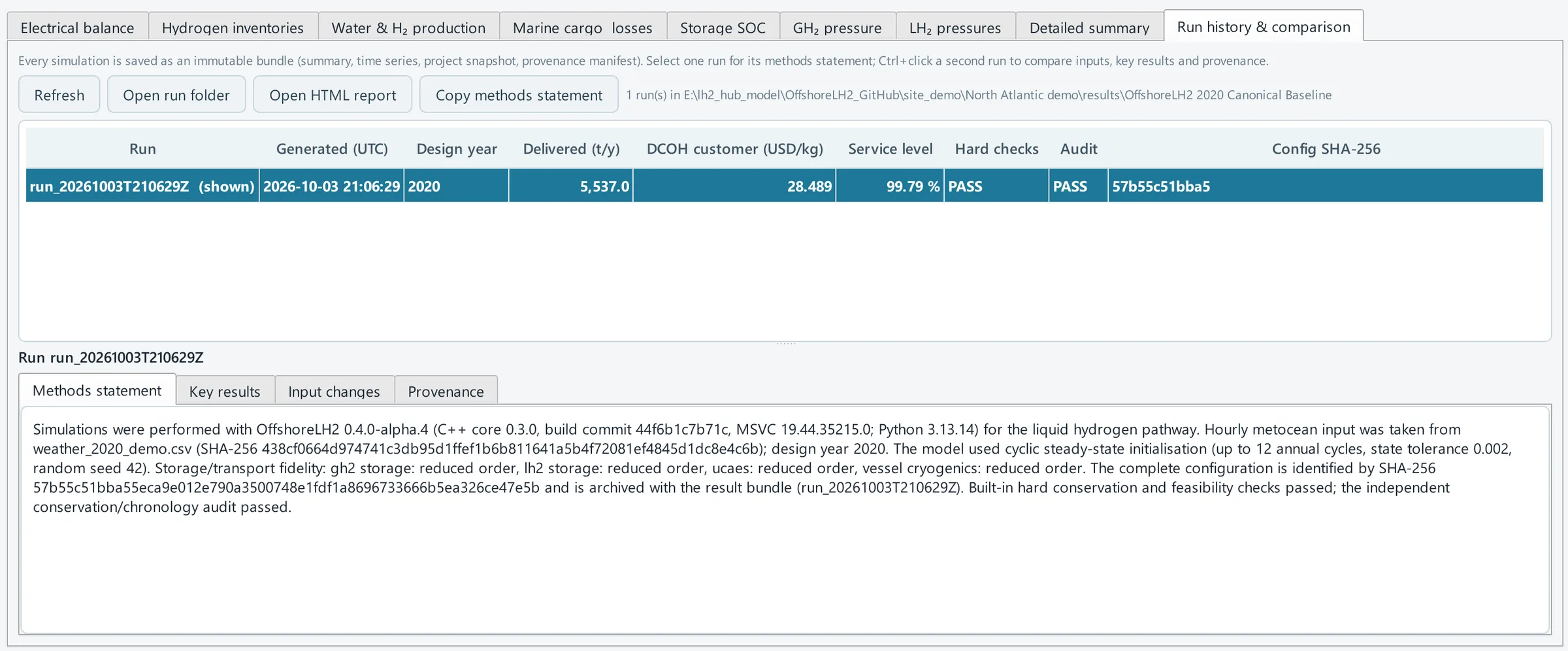
Every simulation is saved automatically as an unchangeable bundle in results/<project>/run_<time>/, next to the project file. The Run history & comparison tab lists them with key results, check outcomes and a configuration hash.
Select one run to see its methods statement, a citation-ready paragraph generated only from what was recorded: software and core versions, build commit, weather file and its hash, simulation mode and seed, fidelity, and check outcomes. Copy methods statement puts it on the clipboard.
Ctrl+click a second run to compare key results (difference and relative change), input changes and provenance.
A saved run with its generated methods statement.
12
Explore with the Research Lab
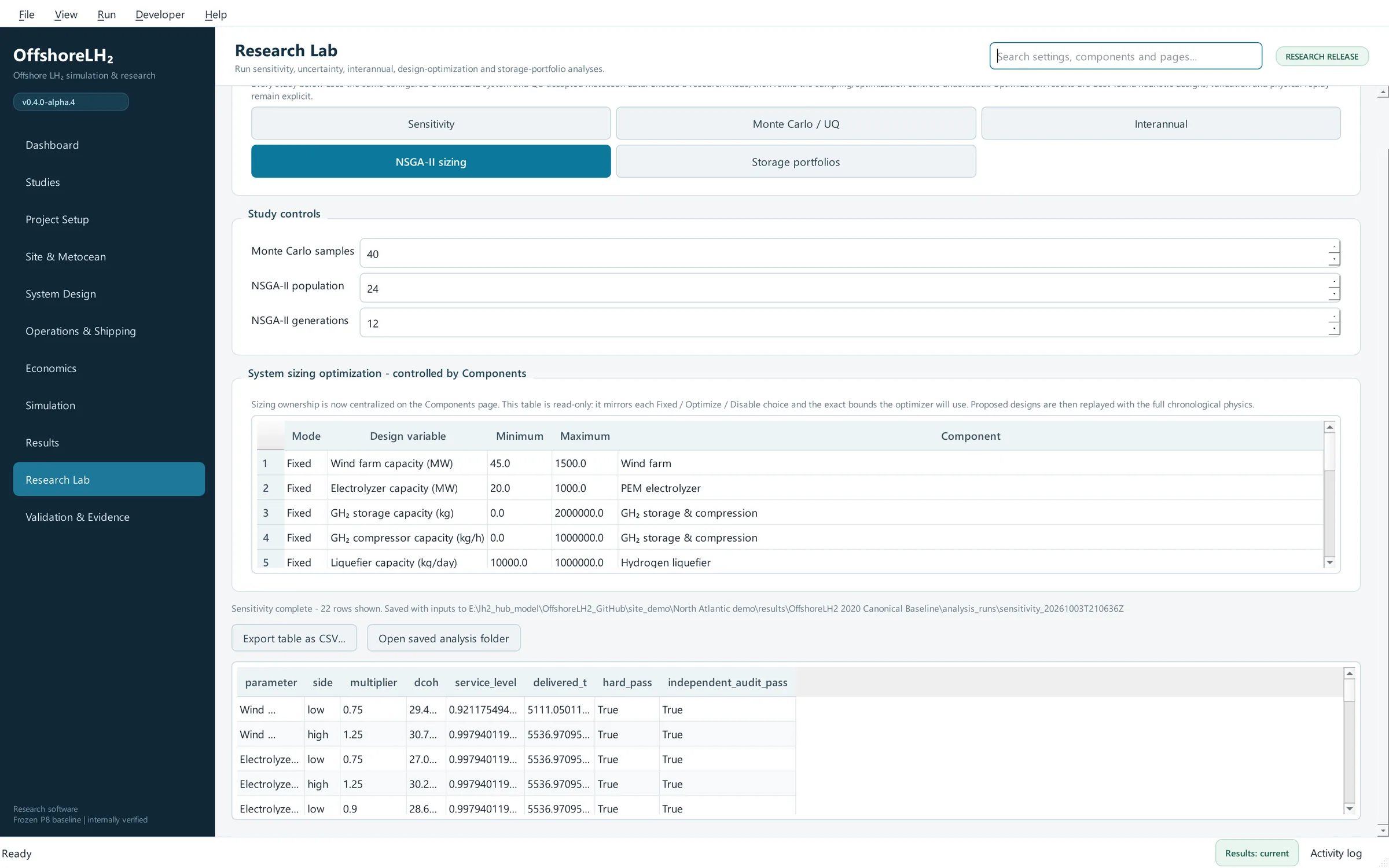
The Research Lab runs many simulations through the same physics to answer "what if" questions. Choose a mode:
Sensitivity: changes one input at a time, up and down, and shows the effect on cost, service and delivery.
Monte Carlo / UQ: samples declared uncertainties together (Latin hypercube) to show the spread of outcomes.
Interannual: runs every accepted weather year separately, so year-to-year variability stays visible.
NSGA-II sizing: searches the components set to Optimize for the best trade-offs between cost and delivery. Proposed designs are replayed with the full physics.
Storage portfolios: compares no storage, battery, compressed air and both, on the same basis.
Each finished analysis is saved in analysis_runs with its table and an analysis_context.json that records the seed, settings, weather hash and project snapshot. Export table as CSV saves the displayed table.
Remember. Optimization returns best-found designs within your bounds, not a proven global optimum. Rerun important designs on complete weather years, with the appropriate fidelity, before drawing conclusions.
Research Lab after a sensitivity study. Every row is a full simulation with its own checks.
13
Work with Studies
A study turns a research question into saved, repeatable experiments. Your project still defines the physical system; the study defines what to test with it.
New Study from Project creates a draft study that refers to your saved .olh2 project.
Published studies rerun an earlier study's workflow under its original assumptions, or with current physics.
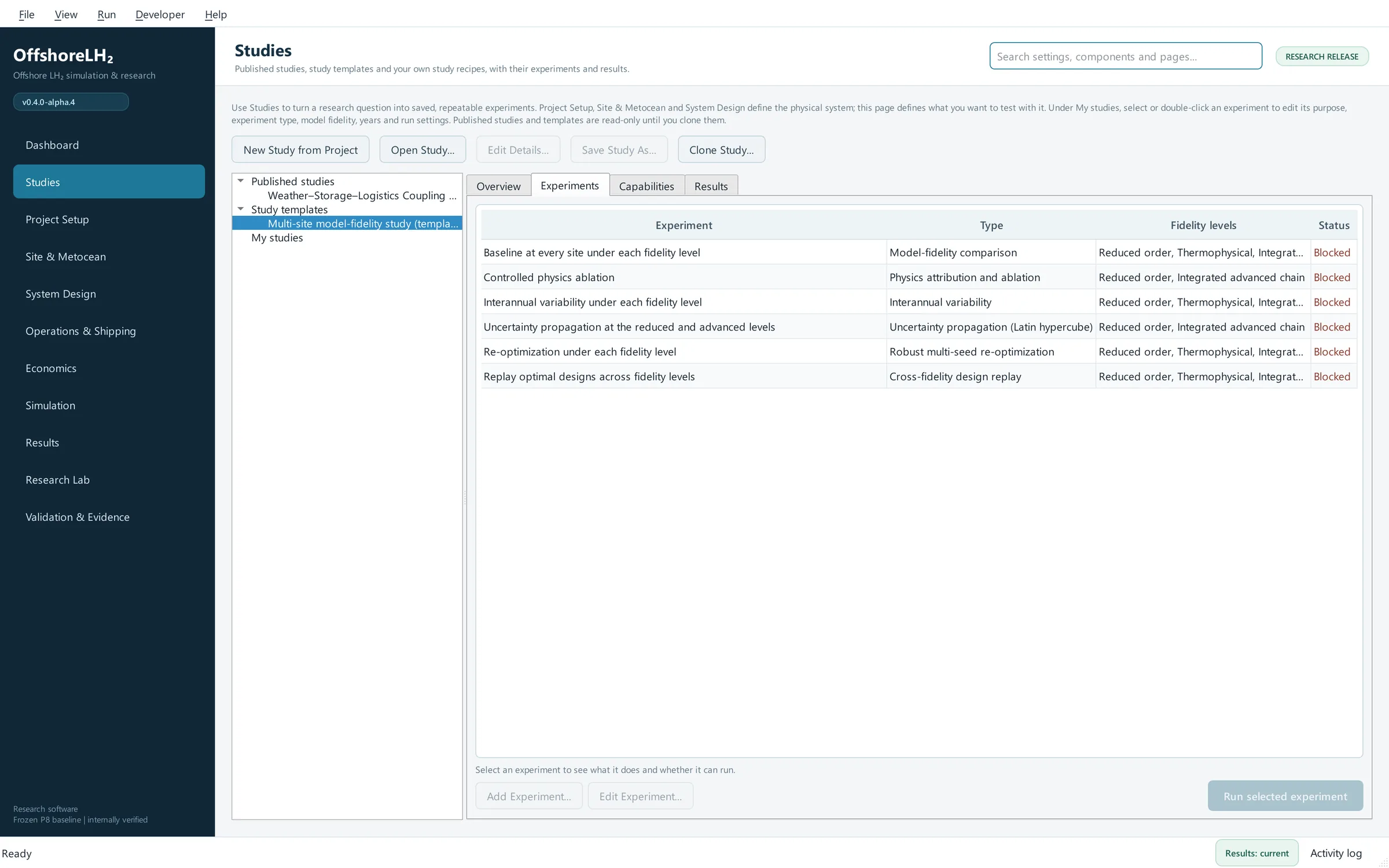
Study templates, such as the multi-site model-fidelity template, show how a larger study is laid out. Clone one and fill in its sites and data.
The Experiments tab marks each experiment Ready, Declared or Blocked, with the reason. Only Ready experiments run.
The Capabilities tab shows the status of every technology and method the study uses.
Study runs are written to results/<project>/study_runs/ with a manifest of inputs and hashes, and never overwrite earlier runs.
A study template lists its experiments. They stay blocked until the template's sites and data are filled in.
14
Export and share
Export latest results on the Simulation page (or File → Export Results) writes a complete bundle:
summary.json: key results, economics and checks;
timeseries.csv: the hourly output;
report.html: a portable report you can open in any browser;
project_snapshot.json: the exact configuration used;
manifest.json: software version, core version, build commit and SHA-256 hashes of the configuration and weather data.
To let someone else reproduce a result, share the .olh2 project, the weather file and the manifest.
15
Interpret results responsibly
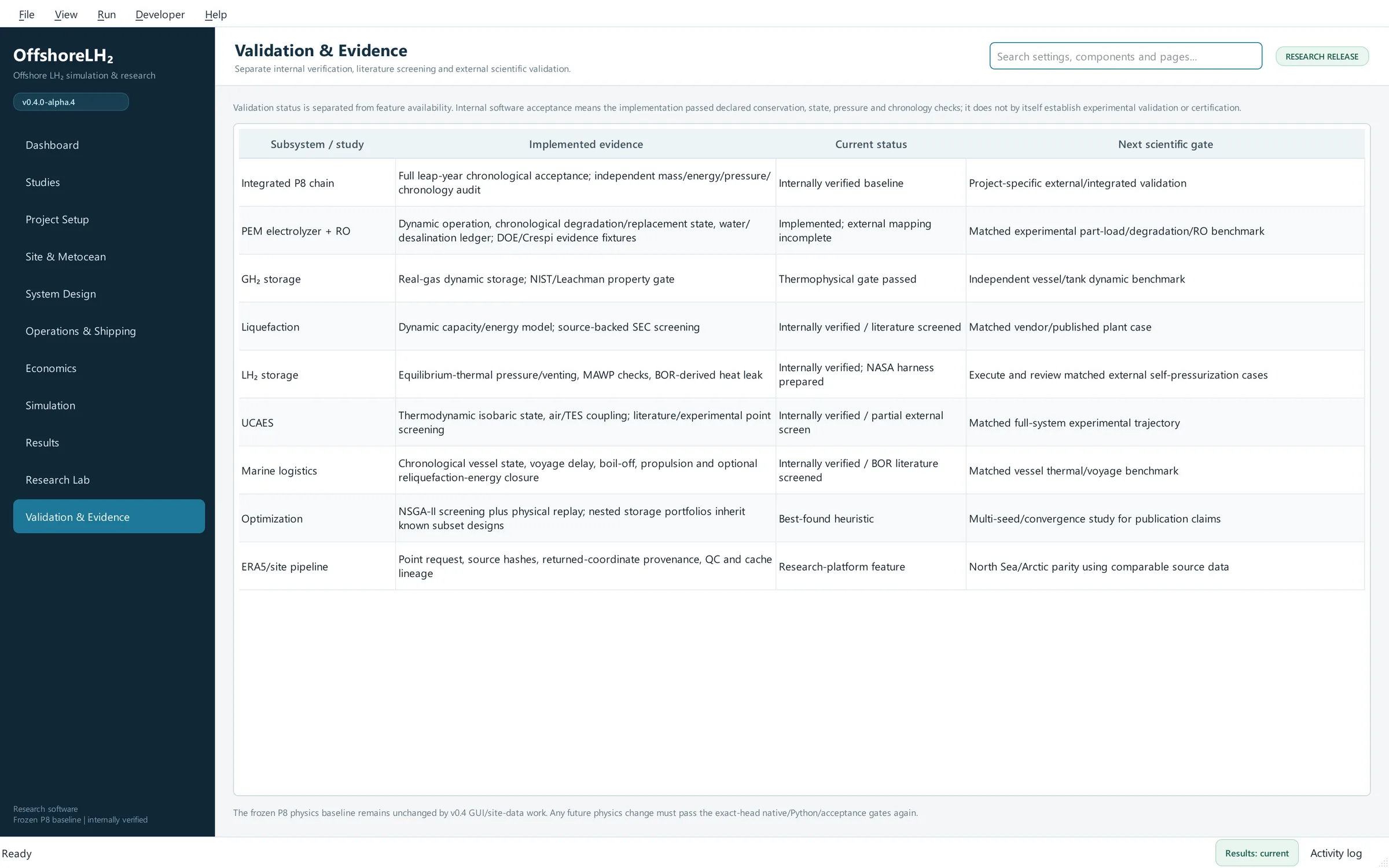
The Validation & Evidence page states, for each subsystem, what has been verified internally, what has been screened against literature and what still needs external validation. Keep three distinctions in mind:
Passing the conservation and feasibility checks shows the simulation is internally consistent, not that every assumption is right.
Higher fidelity means more physical detail, not independent validation.
Default costs are study assumptions, not market prices or quotes.
Validation & Evidence: what each subsystem's results can and cannot support.
16
Command line and Python
The desktop application is optional. The same engine runs without a graphical interface, which is useful for batch work and continuous integration:
# run a saved project and write its result bundle
offshorelh2 run examples/canonical_baseline_2020.olh2 --output results/baseline_2020

# download and transform ERA5 point weather for complete years
offshorelh2 acquire-era5 --lat 45.0 --lon -60.0 --first-year 2020 --last-year 2020

# compare two canonical weather CSV files
offshorelh2 weather-parity reference.csv candidate.csv
From Python, the OffshoreH2Model class runs a pathway directly on a quality-checked weather table:
from offshore_lh2 import OffshoreH2Model, pipeline_core_config

model = OffshoreH2Model("gaseous_pipeline", pipeline_core_config())
bundle = model.simulate_dataframe(accepted_weather, economics=True)
17
Shortcuts, terms and common fixes
Keyboard shortcuts
Keys
Action
Ctrl+N / Ctrl+O / Ctrl+S
New, open and save a project
Ctrl+F or Ctrl+K
Search settings, components and pages
Ctrl+1 … Ctrl+9
Open the first nine pages in the sidebar
F5 / Shift+F5
Run the simulation / cancel the running computation
Ctrl+L
Show or hide the Activity log
Key terms
DCOH
Delivered cost of hydrogen: annualized system cost divided by the hydrogen delivered, in US dollars per kilogram, at a stated boundary.
Service level
Hydrogen actually delivered as a share of the hydrogen requested by the customer.
GH₂ / LH₂
Gaseous and liquid hydrogen. Liquid hydrogen is stored at about −253 °C, and some of it boils off as heat leaks in.
UCAES
Underwater compressed-air energy storage: air stored at the pressure of the surrounding water.
ERA5
The ECMWF global atmospheric reanalysis, with hourly wind and wave data from 1940 onwards, distributed through the Copernicus Climate Data Store.
Operability
The share of time in which wind and wave conditions allow cargo transfer.
Reduced-order model
A faster, simplified representation that prescribes or averages behaviour instead of resolving every physical state.
Cyclic steady state
A design year repeated until the storage levels at its start and end agree.
NSGA-II
A genetic algorithm that searches for designs balancing several objectives at once, such as cost and delivery.
Common fixes
"Weather file missing or moved." Choose the file again on Site & Metocean, or save the project next to its weather file.
Cyclic steady state with electrolyzer ageing. These cannot be combined. Untick "Solve cyclic initial state" for a finite chronological run; the readiness list offers a Go to button.
Results marked stale. An input changed after the run. Run again before exporting.
A pathway cannot be selected. It is research-stage and is disabled until it passes its release gates.
A run is taking long. Higher-fidelity years take about a minute each. Use Cancel run; the window stays responsive.